

If you came from my Introduction to Machine Learning, you will have a high-level understanding of Supervised Learning and Machine Learning. If not, click the link above, like and subscribe... oh wait wrong platform. You can also read the next section for a quick recap before we dive deeper.
Supervised Learning Recap
Supervised Learning is a machine learning algorithm that uses labeled data to train a model. Labeled data means the input and output data is already known and the model will map the input data to the output data.
An example of Supervised Learning is Regression, which is what we will be focusing on in this article. Regression is where we use continuous data (where the numbers can be anything along a range like temperature or house prices) to train a model and predict a continuous value based on a new input. Let's go into detail with concrete examples.
Regression
In short, regression helps us find relationships between input data and output data so that we can start making predictions on new data. There are different kinds of regression, some of which I will describe below.
Types of Regression
Simple Linear Regression: The straight line fit for one input field and its output. Imagine you have data on a graph and you took a ruler and needed to draw a straight line through most of the data points. We will go into more detail later, however, data is never this simple. Let's look at a more realistic scenario.
Multi-Variate Regression: In the real world, data is complex and rarely simple (just like life, things get complicated). We often need multiple input fields to build a stronger relationship with its output. Think of the relationship with your partner, to build a strong relationship, there are multiple inputs needed (some more important than others but all still needed) to strengthen that relationship and predict a long-term outcome together. Oh no, did I just assume your relationship status... Moving along to Logistic Regression and pretend that never happened.
Logistic Regression: The yes/no algorithm. If you recall from my previous article (if you haven't read it yet, I am only slightly disappointed) we spoke about an algorithm called classification and gave an example of an application identifying if a picture contains a hotdog or not. Logistic Regression can be used for classifying data into one of two categories.
There are many more types of Regression, but for this article, I want to focus on Simple Linear Regression. Let's take a closer look.
Simple Linear Regression - Drawing Straight Lines
Simple Linear Regression is best explained through examples. Let's have a look at the dataset below. Here we have a dataset showing the size of a house in square meters and its price for a given area in South Africa.
| House Size (square meters) | House Price (ZAR) |
| 111.48 | 2,025,000 |
| 144 | 2,610,000 |
| 79 | 1,530,000 |
| 157.94 | 2,880,000 |
| 222.97 | 4,050,000 |
| 92.9 | 1,755,000 |
| 130.06 | 2,250,000 |
| 195.1 | 3,420,000 |
| 88.26 | 1,620,000 |
| 171.87 | 3,150,000 |
Looking at the table of data, it's difficult to interpret or understand any type of relationship. Visualizing the data will give you a better understanding, and who doesn't like pictures over numbers?
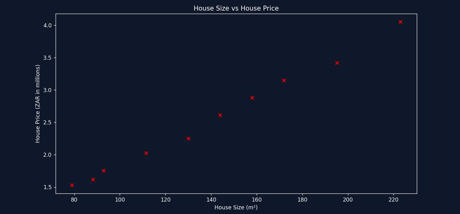
Here we see the dataset visualized using a scatter plot. See the pattern? We can immediately identify a trend that as the house size increases, the more expensive it is. This makes sense because the data was collected for the same area. There's a possibility that if the data was collected for multiple areas, a smaller house in one area could be more expensive than a bigger house in a different area. For simplicity, we used a dataset for a single area to illustrate the relationship between house size and house price. Using this dataset and visualization, we can quickly interpret the data and make an educated guess at predicting a new value. For example, a house size of 100 square meters would cost about R2,000,000.
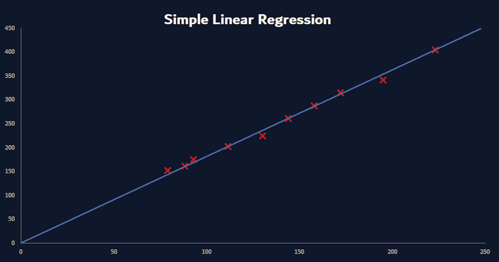
Without you knowing it, we intuitively used something like Linear Regression to predict a house price based on house size. Let's visualize how we were able to accomplish this.

We imagined a straight line through the data points trying to get the line to touch as many points as possible. In a nutshell, this is the core idea behind Simple Linear Regression. A simple example like this was able to illustrate an important concept. Unfortunately, real-world use cases are never this simple. Datasets often have multiple inputs that affect the output, for example: house size, number of bedrooms, area, garage size etc. Having this many fields makes visualizing and intuitively interpreting the data impossible. Linear Regression gives us a strategy to solve this problem and find the best possible fit for a straight line.
Warning! Warning! Mathematics ahead, x's and y's may cause tears to be shed!
A linear relationship and drawing a straight line are both represented by the formula below.
$$y = mx + b$$
y is the output we want to predict (House Price).
m represents the slope of the line: This tells us how much the house price (y-axis) changes as the house size (x-axis) increases by 1. Think of it like the steepness of the line. A steeper slope means the price goes up much faster with each square meter of house size.
x represents the input (House Size).
b represents the Y-intercept: This is the starting point of the line on the price (y-axis) when the house size (x-axis) is zero. It helps us position the line up and down on the price graph.
We can adjust values for m and b to best fit the relationship of x and y. We can try guessing good values for m and b as seen below, but that would take forever.
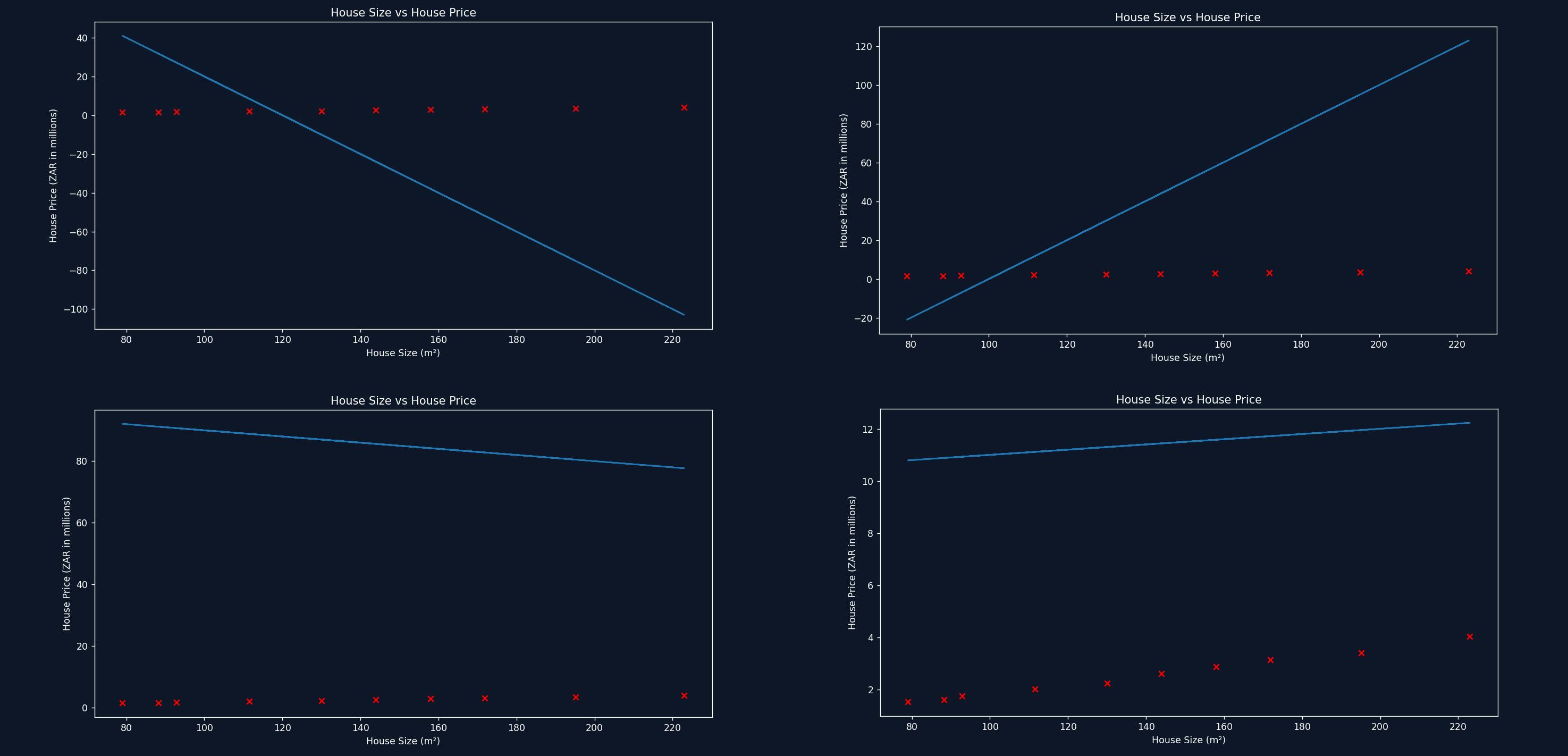
These lines aren't great fits. But how could we be sure we've found the best possible line? We do this by measuring the error between the straight line and the values from our dataset.

We can see above, the white dotted line representing the errors for each value in the dataset. We square the error (so that negative error values do not cancel out the positive error values) and add them together. Then we divide the sum by the number of data points to get a value that represents how well our line fits the data. This is called the cost function and is represented by the following formula.
$$\displaystyle\frac{1}{2n}\sum\limits_{i=1}^{n}(House Price[i] - PredictedValue)^2$$
Now that we have defined the cost function, we need to try and determine the smallest possible error. Unfortunately, it's not always possible for the error to be exactly 0 unless the dataset is a perfect straight line. Remember, real-world data is messy, so we're aiming for the best possible approximation, not perfection.
So how do we find the best possible values for slope (m) and y-intercept (b) to minimize the error? We do this by taking the partial derivative of the cost function with respect to m and then b. Yikes! Partial derivative? I will try to keep it simple, but for those interested in the math, see below for some resources.
Let's break it down bit by bit – don't worry, it's less scary than it sounds! Essentially, derivatives help us find how to tweak an equation to improve the results. Since we're adjusting both the m and b of our line, we need partial derivatives to handle them one at a time. This leaves us with 2 equations. Using these 2 equations, we start running the calculations repeatedly, tweaking m and b hundreds, sometimes thousands of times. Each iteration takes a small step trying to minimize the error. Don't worry, the computer does this quickly! For simplicity, imagine we only optimize for slope (m). Gradient descent would look like this.

See how on each calculation, it takes a small step to decrease the error and find the optimal value for m. Now let's take a look at plotting the straight line each time as gradient descent tweaks the values for both m and b.
See the line improving with each step? That's the power of gradient descent! In the end, it finds the best values for m and b to represent the relationship between House Size and House Price, allowing us to make approximate predictions for any size home.
Remember, even this simple case had some complexity! When increasing the number of inputs, this technique becomes essential for finding the best solution.
Conclusion
We started with a messy table of numbers, drew straight lines, wrestled with some math, and even witnessed an epic GIF battle. We have emerged victorious in our quest to establish a fundamental understanding of Simple Linear Regression. If that's not worthy of a celebratory nap, I don't know what is. GGWP (Good Game Well Played) to surviving Simple Linear Regression, may your data always be tidy and your lines forever straight!